Bike Sharing Demand
공유 자전거 사용량 예측
공유 자전거 사용량 예측 [Kaggle]
목표
- 워싱턴 D.C.의 Capital Bikeshare 수요를 시간대 별로 예측
- 자전거 대여 수요를 예측하기 위해 과거 사용 패턴과 날씨 데이터를 분석
데이터 필드
- 과거 사용 패턴: 시간(hour), 휴일 여부
- 날씨 데이터: 계절, 날씨, 온도, 체감 온도, 습도, 풍속
| 필드 | 내용 |
|---|---|
datetime |
날짜 + 시간 타임스탬프 |
season |
1: 봄, 2: 여름, 3: 가을, 4: 겨울 |
holiday |
휴일 여부 |
weateher |
1: Clear, Few clouds, Partly cloudy, Partly cloudy 2: Mist + Cloudy, Mist + Broken clouds, Mist + Few clouds, Mist 3: Light Snow, Light Rain + Thunderstorm + Scattered clouds, Light Rain + Scattered clouds 4: Heavy Rain + Ice Pallets + Thunderstorm + Mist, Snow + Fog |
temp |
섭씨 온도 |
atemp |
섭씨 체감 온도 |
humidity |
습도 |
windspeed |
풍속 |
casual |
비회원 대여량 |
registered |
회원 대여량 |
count |
총 대여량 |
casual, registered, count 필드를 예측해야 한다.
EDA & 예측
라이브러리 로드
import pandas as pd
import numpy as np
import matplotlib.pyplot as plt
import seaborn as sns
from scipy import stats
%matplotlib inline
plt.rc("font", family="Malgun Gothic")
데이터셋 로드
## This Python 3 environment comes with many helpful analytics libraries installed
## It is defined by the kaggle/python Docker image: https://github.com/kaggle/docker-python
## For example, here's several helpful packages to load

import numpy as np ## linear algebra
import pandas as pd ## data processing, CSV file I/O (e.g. pd.read_csv)

## Input data files are available in the read-only "../input/" directory
## For example, running this (by clicking run or pressing Shift+Enter) will list all files under the input directory

import os
for dirname, _, filenames in os.walk('/kaggle/input'):
    for filename in filenames:
        print(os.path.join(dirname, filename))

## You can write up to 20GB to the current directory (/kaggle/working/) that gets preserved as output when you create a version using "Save & Run All"
## You can also write temporary files to /kaggle/temp/, but they won't be saved outside of the current session
/kaggle/input/bike-sharing-demand/sampleSubmission.csv
/kaggle/input/bike-sharing-demand/train.csv
/kaggle/input/bike-sharing-demand/test.csv
train = pd.read_csv("/kaggle/input/bike-sharing-demand/train.csv", parse_dates=['datetime'])
test = pd.read_csv("/kaggle/input/bike-sharing-demand/test.csv", parse_dates=['datetime'])
sample = pd.read_csv("/kaggle/input/bike-sharing-demand/sampleSubmission.csv", parse_dates=['datetime'])
데이터셋 요약
데이터 Shape
print(train.shape, test.shape, sample.shape)
(10886, 12) (6493, 9) (6493, 2)
데이터 필드
train.info()
<class 'pandas.core.frame.DataFrame'>
RangeIndex: 10886 entries, 0 to 10885
Data columns (total 12 columns):
 ##   Column      Non-Null Count  Dtype
---  ------      --------------  -----
 0   datetime    10886 non-null  datetime64[ns]
 1   season      10886 non-null  int64
 2   holiday     10886 non-null  int64
 3   workingday  10886 non-null  int64
 4   weather     10886 non-null  int64
 5   temp        10886 non-null  float64
 6   atemp       10886 non-null  float64
 7   humidity    10886 non-null  int64
 8   windspeed   10886 non-null  float64
 9   casual      10886 non-null  int64
 10  registered  10886 non-null  int64
 11  count       10886 non-null  int64
dtypes: datetime64[ns](1), float64(3), int64(8)
memory usage: 1020.7 KB
test.info()
<class 'pandas.core.frame.DataFrame'>
RangeIndex: 6493 entries, 0 to 6492
Data columns (total 9 columns):
 ##   Column      Non-Null Count  Dtype
---  ------      --------------  -----
 0   datetime    6493 non-null   datetime64[ns]
 1   season      6493 non-null   int64
 2   holiday     6493 non-null   int64
 3   workingday  6493 non-null   int64
 4   weather     6493 non-null   int64
 5   temp        6493 non-null   float64
 6   atemp       6493 non-null   float64
 7   humidity    6493 non-null   int64
 8   windspeed   6493 non-null   float64
dtypes: datetime64[ns](1), float64(3), int64(5)
memory usage: 456.7 KB
학습 데이터에 존재하는 casual, registered, count 필드가 테스트 데이터에는 없다.
sampleSubmission.csv에 따르면 날짜 및 시간대 별로 count를 예측해야 한다.
데이터 샘플
train.head()
| datetime | season | holiday | workingday | weather | temp | atemp | humidity | windspeed | casual | registered | count | |
|---|---|---|---|---|---|---|---|---|---|---|---|---|
| 0 | 2011-01-01 00:00:00 | 1 | 0 | 0 | 1 | 9.84 | 14.395 | 81 | 0.0 | 3 | 13 | 16 |
| 1 | 2011-01-01 01:00:00 | 1 | 0 | 0 | 1 | 9.02 | 13.635 | 80 | 0.0 | 8 | 32 | 40 |
| 2 | 2011-01-01 02:00:00 | 1 | 0 | 0 | 1 | 9.02 | 13.635 | 80 | 0.0 | 5 | 27 | 32 |
| 3 | 2011-01-01 03:00:00 | 1 | 0 | 0 | 1 | 9.84 | 14.395 | 75 | 0.0 | 3 | 10 | 13 |
| 4 | 2011-01-01 04:00:00 | 1 | 0 | 0 | 1 | 9.84 | 14.395 | 75 | 0.0 | 0 | 1 | 1 |
결측치 확인
train.isnull().sum()
datetime      0
season        0
holiday       0
workingday    0
weather       0
temp          0
atemp         0
humidity      0
windspeed     0
casual        0
registered    0
count         0
dtype: int64
test.isnull().sum()
datetime      0
season        0
holiday       0
workingday    0
weather       0
temp          0
atemp         0
humidity      0
windspeed     0
dtype: int64
fig, (ax1, ax2, ax3, ax4) = plt.subplots(ncols=4)
fig.set_size_inches(20, 10)
sns.regplot(data=train, x='temp', y='count', ax=ax1)
sns.regplot(data=train, x='atemp', y='count', ax=ax2)
sns.regplot(data=train, x='windspeed', y='count', ax=ax3)
sns.regplot(data=train, x='humidity', y='count', ax=ax4)
<AxesSubplot:xlabel='humidity', ylabel='count'>
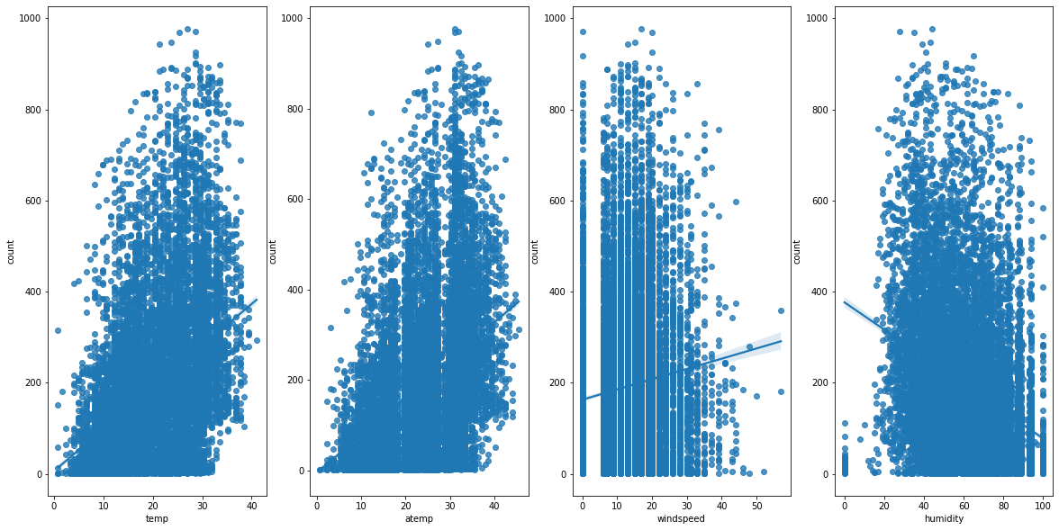
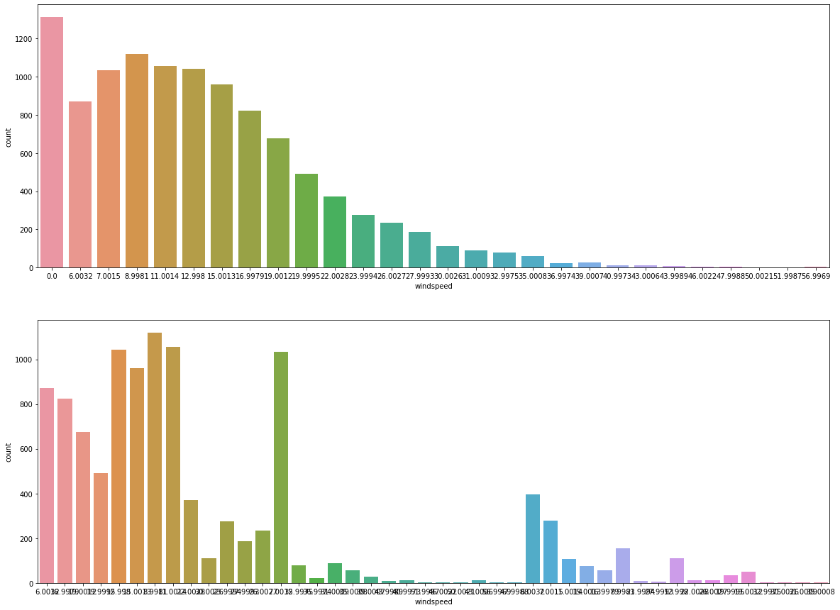
print(len(train[train['windspeed'] == 0]), str(len(train[train['windspeed'] == 0])/len(train)*100)+"%")
1313 12.061363218813154%
windspeed의 약 12%가 0에 분포하며, 다음 구간에 분포가 비어 있다.
결측치가 0으로 기입되어 있다고 가정할 수 있다.
EDA
시기별 대여량
def build_datetime_features(df):
    ## 날짜 및 시간 피처 생성
    df['season_str'] = df['season'].map({1: "Spring", 2: "Summer", 3: "Fall", 4: "Winter"})
    df['year'] = df['datetime'].dt.year
    df['month'] = df['datetime'].dt.month
    df['day'] = df['datetime'].dt.day
    df['weekday'] = df['datetime'].dt.dayofweek
    df['hour'] = df['datetime'].dt.hour
    return df
train = build_datetime_features(train)
train.head()
| datetime | season | holiday | workingday | weather | temp | atemp | humidity | windspeed | casual | registered | count | season_str | year | month | day | weekday | hour | |
|---|---|---|---|---|---|---|---|---|---|---|---|---|---|---|---|---|---|---|
| 0 | 2011-01-01 00:00:00 | 1 | 0 | 0 | 1 | 9.84 | 14.395 | 81 | 0.0 | 3 | 13 | 16 | Spring | 2011 | 1 | 1 | 5 | 0 |
| 1 | 2011-01-01 01:00:00 | 1 | 0 | 0 | 1 | 9.02 | 13.635 | 80 | 0.0 | 8 | 32 | 40 | Spring | 2011 | 1 | 1 | 5 | 1 |
| 2 | 2011-01-01 02:00:00 | 1 | 0 | 0 | 1 | 9.02 | 13.635 | 80 | 0.0 | 5 | 27 | 32 | Spring | 2011 | 1 | 1 | 5 | 2 |
| 3 | 2011-01-01 03:00:00 | 1 | 0 | 0 | 1 | 9.84 | 14.395 | 75 | 0.0 | 3 | 10 | 13 | Spring | 2011 | 1 | 1 | 5 | 3 |
| 4 | 2011-01-01 04:00:00 | 1 | 0 | 0 | 1 | 9.84 | 14.395 | 75 | 0.0 | 0 | 1 | 1 | Spring | 2011 | 1 | 1 | 5 | 4 |
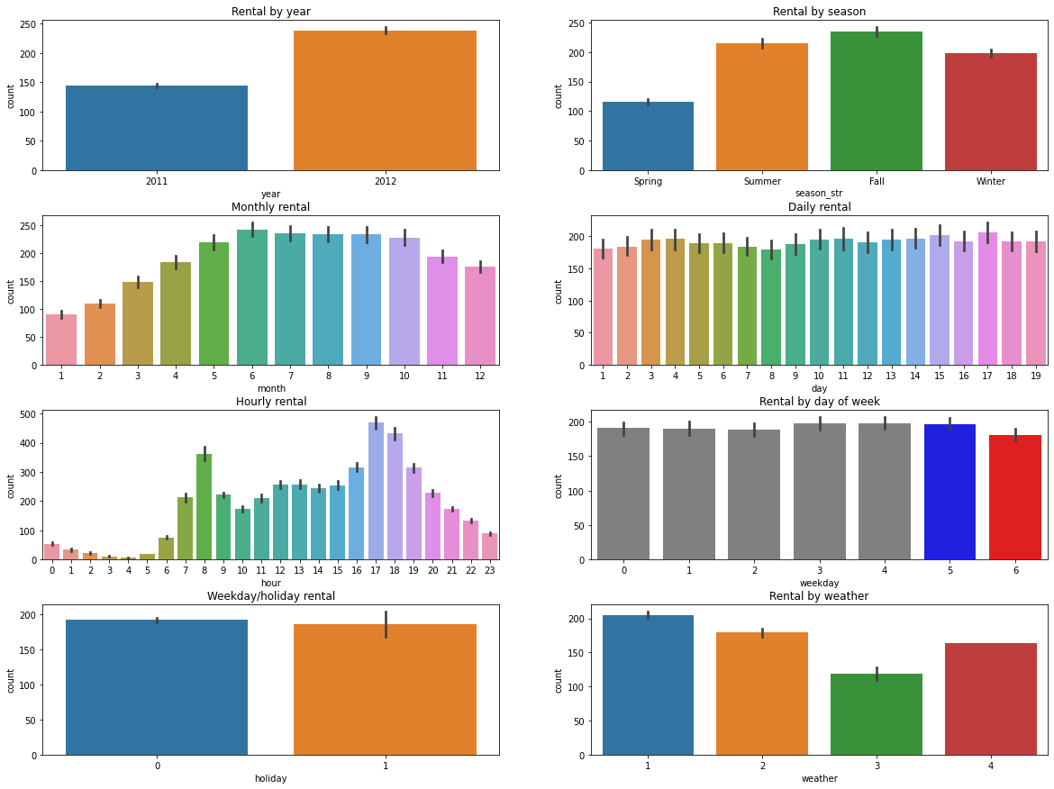
## Barplot
fig, ((ax1, ax2), (ax3, ax4), (ax5, ax6), (ax7, ax8)) = plt.subplots(nrows=4, ncols=2)
fig.set_size_inches(20, 15)
plt.subplots_adjust(wspace=0.2, hspace=0.3)

ax1.set(title="Rental by year")
sns.barplot(data=train, x='year', y='count', orient='v', ax=ax1)

ax2.set(title="Rental by season")
sns.barplot(data=train, x='season_str', y='count', ax=ax2)

ax3.set(title="Monthly rental")
sns.barplot(data=train, x='month', y='count', ax=ax3)

ax4.set(title="Daily rental")
sns.barplot(data=train, x='day', y='count', ax=ax4)

ax5.set(title="Hourly rental")
sns.barplot(data=train, x='hour', y='count', ax=ax5)

ax6.set(title="Rental by day of week")
sns.barplot(data=train, x='weekday', y='count', ax=ax6,
            palette=['gray', 'gray', 'gray', 'gray', 'gray', 'blue', 'red'])

ax7.set(title="Weekday/holiday rental")
sns.barplot(data=train, x='holiday', y='count', ax=ax7)

ax8.set(title="Rental by weather")
sns.barplot(data=train, x='weather', y='count', ax=ax8)
<AxesSubplot:title={'center':'Rental by weather'}, xlabel='weather', ylabel='count'>
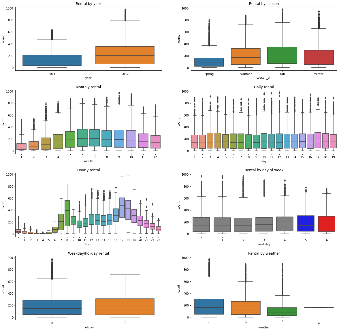
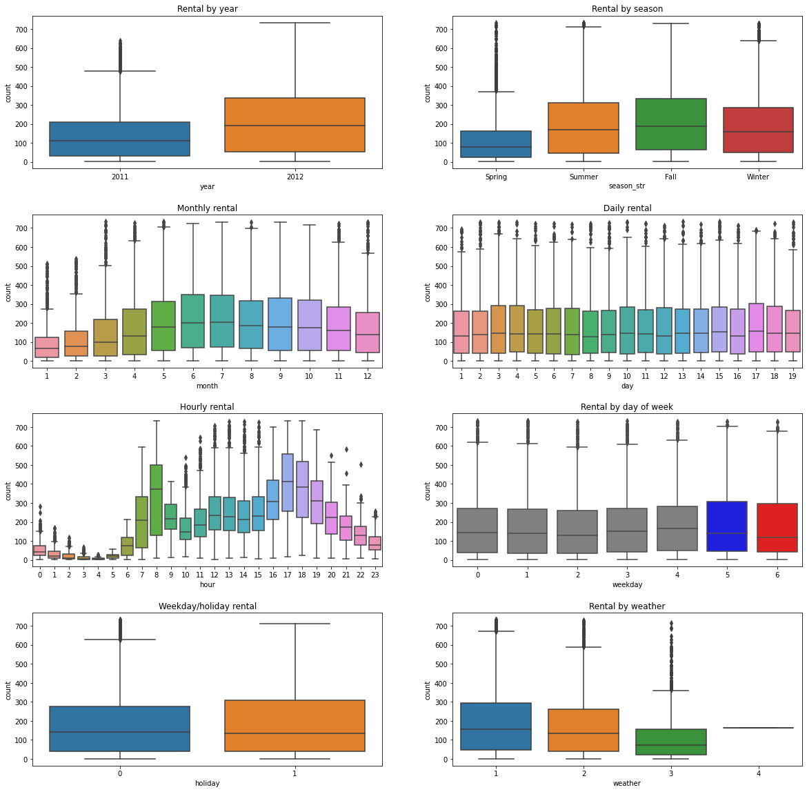
## Boxplot
fig, ((ax1, ax2), (ax3, ax4), (ax5, ax6), (ax7, ax8)) = plt.subplots(nrows=4, ncols=2)
fig.set_size_inches(20, 20)
plt.subplots_adjust(wspace=0.2, hspace=0.3)

ax1.set(title="Rental by year")
sns.boxplot(data=train, x='year', y='count', ax=ax1)

ax2.set(title="Rental by season")
sns.boxplot(data=train, x='season_str', y='count', ax=ax2)

ax3.set(title="Monthly rental")
sns.boxplot(data=train, x='month', y='count', ax=ax3)

ax4.set(title="Daily rental")
sns.boxplot(data=train, x='day', y='count', ax=ax4)

ax5.set(title="Hourly rental")
sns.boxplot(data=train, x='hour', y='count', ax=ax5)

ax6.set(title="Rental by day of week")
sns.boxplot(data=train, x='weekday', y='count', ax=ax6,
            palette=['gray', 'gray', 'gray', 'gray', 'gray', 'blue', 'red'])

ax7.set(title="Weekday/holiday rental")
sns.boxplot(data=train, x='holiday', y='count', ax=ax7)

ax8.set(title="Rental by weather")
sns.boxplot(data=train, x='weather', y='count', ax=ax8)
<AxesSubplot:title={'center':'Rental by weather'}, xlabel='weather', ylabel='count'>
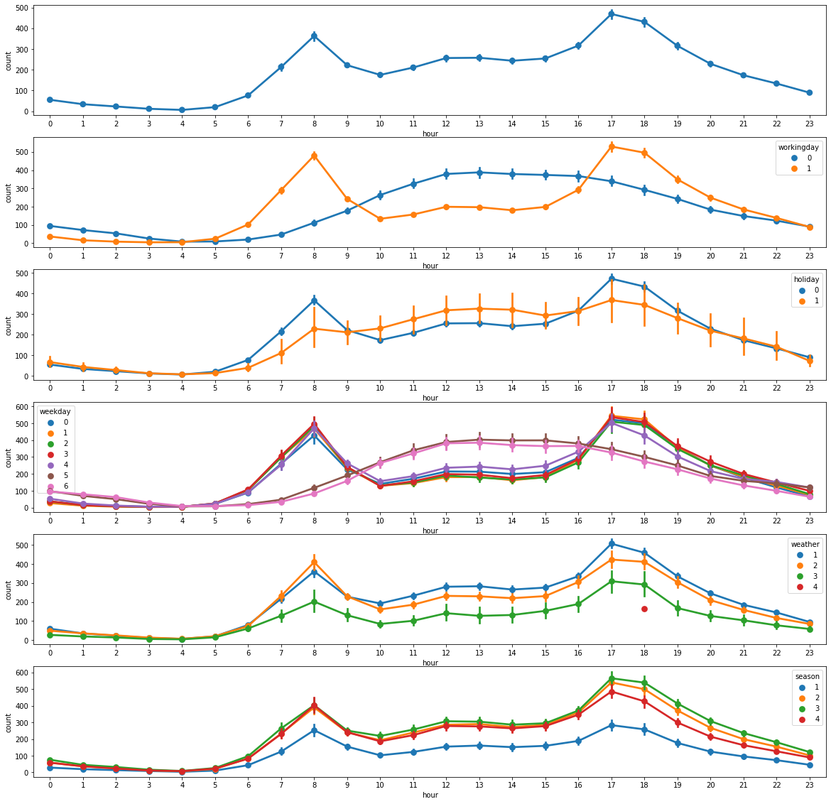
## 시간대별 대여량
fig, (ax1, ax2, ax3, ax4, ax5, ax6) = plt.subplots(nrows=6)
fig.set_size_inches(20, 20)

sns.pointplot(data=train, x='hour', y='count', ax=ax1)
sns.pointplot(data=train, x='hour', y='count', hue='workingday', ax=ax2)
sns.pointplot(data=train, x='hour', y='count', hue='holiday', ax=ax3)
sns.pointplot(data=train, x='hour', y='count', hue='weekday', ax=ax4)
sns.pointplot(data=train, x='hour', y='count', hue='weather', ax=ax5)
sns.pointplot(data=train, x='hour', y='count', hue='season', ax=ax6)
<AxesSubplot:xlabel='hour', ylabel='count'>
- 연도별 대여량: 2011 < 2012
- 계절별 대여량: 가을 > 여름 > 겨울 > 봄
- 월별 대여량: 6월 > 7~9월 > 10월 > 5월 > 11월 > 4월 > 12월 > 3월 > 2월 > 1월
- 시간별 대여량: 출퇴근 시간대 대여량과 편차가 큼
- 시기별 대여량:
workingday0과 토요일, 일요일은 비슷한 추세를 보이며, 출퇴근 시간대의 영향을 받지 않음
print(train[train['season'] == 1]['month'].unique())
print(train[train['season'] == 2]['month'].unique())
print(train[train['season'] == 3]['month'].unique())
print(train[train['season'] == 4]['month'].unique())
[1 2 3]
[4 5 6]
[7 8 9]
[10 11 12]
season은 사전적 의미의 계절이 아니라 분기를 의미한다.
이상치 제거
train_normalized = train[np.abs(train['count'] - train['count'].mean()) <= (3*train['count'].std())]
print("Shape of before normalization: ", train.shape)
print("Shape of after normalization: ", train_normalized.shape)
Shape of before normalization:  (10886, 18)
Shape of after normalization:  (10739, 18)
## Boxplot
fig, ((ax1, ax2), (ax3, ax4), (ax5, ax6), (ax7, ax8)) = plt.subplots(nrows=4, ncols=2)
fig.set_size_inches(20, 20)
plt.subplots_adjust(wspace=0.2, hspace=0.3)

ax1.set(title="Rental by year")
sns.boxplot(data=train_normalized, x='year', y='count', ax=ax1)

ax2.set(title="Rental by season")
sns.boxplot(data=train_normalized, x='season_str', y='count', ax=ax2)

ax3.set(title="Monthly rental")
sns.boxplot(data=train_normalized, x='month', y='count', ax=ax3)

ax4.set(title="Daily rental")
sns.boxplot(data=train_normalized, x='day', y='count', ax=ax4)

ax5.set(title="Hourly rental")
sns.boxplot(data=train_normalized, x='hour', y='count', ax=ax5)

ax6.set(title="Rental by day of week")
sns.boxplot(data=train_normalized, x='weekday', y='count', ax=ax6,
            palette=['gray', 'gray', 'gray', 'gray', 'gray', 'blue', 'red'])

ax7.set(title="Weekday/holiday rental")
sns.boxplot(data=train_normalized, x='holiday', y='count', ax=ax7)

ax8.set(title="Rental by weather")
sns.boxplot(data=train_normalized, x='weather', y='count', ax=ax8)
<AxesSubplot:title={'center':'Rental by weather'}, xlabel='weather', ylabel='count'>
결측치 보정
windspeed의 결측치는 0으로 되어 있다. 0인 것들의 windspeed를 예측하여 보정한다.
from sklearn.ensemble import RandomForestClassifier
wind0 = train.loc[train['windspeed'] == 0]
wind_not0 = train.loc[train['windspeed'] != 0]
print("Number of rows with 0 windspeed before prediction: ", len(wind0))
Number of rows with 0 windspeed before prediction: 1313
## windspeed와의 상관계수 절대값 내림차순
corr = wind_not0.corr()[['windspeed']]
corr.rename(columns={'windspeed': 'corr'}, inplace=True)
corr['corr_abs'] = corr['corr'].abs()
corr.sort_values(by='corr_abs', ascending=False)
| corr | corr_abs | |
|---|---|---|
| windspeed | 1.000000 | 1.000000 |
| humidity | -0.328272 | 0.328272 |
| month | -0.142505 | 0.142505 |
| season | -0.138272 | 0.138272 |
| hour | 0.126289 | 0.126289 |
| casual | 0.085342 | 0.085342 |
| count | 0.085014 | 0.085014 |
| registered | 0.073669 | 0.073669 |
| atemp | -0.068576 | 0.068576 |
| temp | -0.038902 | 0.038902 |
| year | -0.035825 | 0.035825 |
| weekday | -0.030849 | 0.030849 |
| workingday | 0.021188 | 0.021188 |
| holiday | 0.015603 | 0.015603 |
| weather | -0.011837 | 0.011837 |
| day | 0.009141 | 0.009141 |
def predict_windspeed(df):
    df_wind0 = df.loc[df['windspeed'] == 0]
    df_wind_not0 = df.loc[df['windspeed'] != 0]

    columns = ['humidity', 'month', 'hour', 'season', 'weather', 'atemp', 'temp']

    rf_model = RandomForestClassifier()
    rf_model.fit(df_wind_not0[columns], df_wind_not0['windspeed'].astype('str'))
    rf_prediction = rf_model.predict(df_wind0[columns])
    df_wind0['windspeed'] = rf_prediction

    result = df_wind_not0.append(df_wind0)
    result.reset_index(inplace=True)
    result.drop('index', inplace=True, axis=1)

    return result
train_before_wind = train.copy()
train = predict_windspeed(train)
/opt/conda/lib/python3.7/site-packages/ipykernel_launcher.py:10: SettingWithCopyWarning:
A value is trying to be set on a copy of a slice from a DataFrame.
Try using .loc[row_indexer,col_indexer] = value instead

See the caveats in the documentation: https://pandas.pydata.org/pandas-docs/stable/user_guide/indexing.html#returning-a-view-versus-a-copy
  ## Remove the CWD from sys.path while we load stuff.
print("Number of rows with 0 windspeed after prediction: ", len(train[train['windspeed'] == 0]))
Number of rows with 0 windspeed after prediction: 0
fig, (ax1, ax2) = plt.subplots(nrows=2)
fig.set_size_inches(20, 15)

sns.countplot(data=train_before_wind, x='windspeed', ax=ax1)
sns.countplot(data=train, x='windspeed', ax=ax2)
<AxesSubplot:xlabel='windspeed', ylabel='count'>
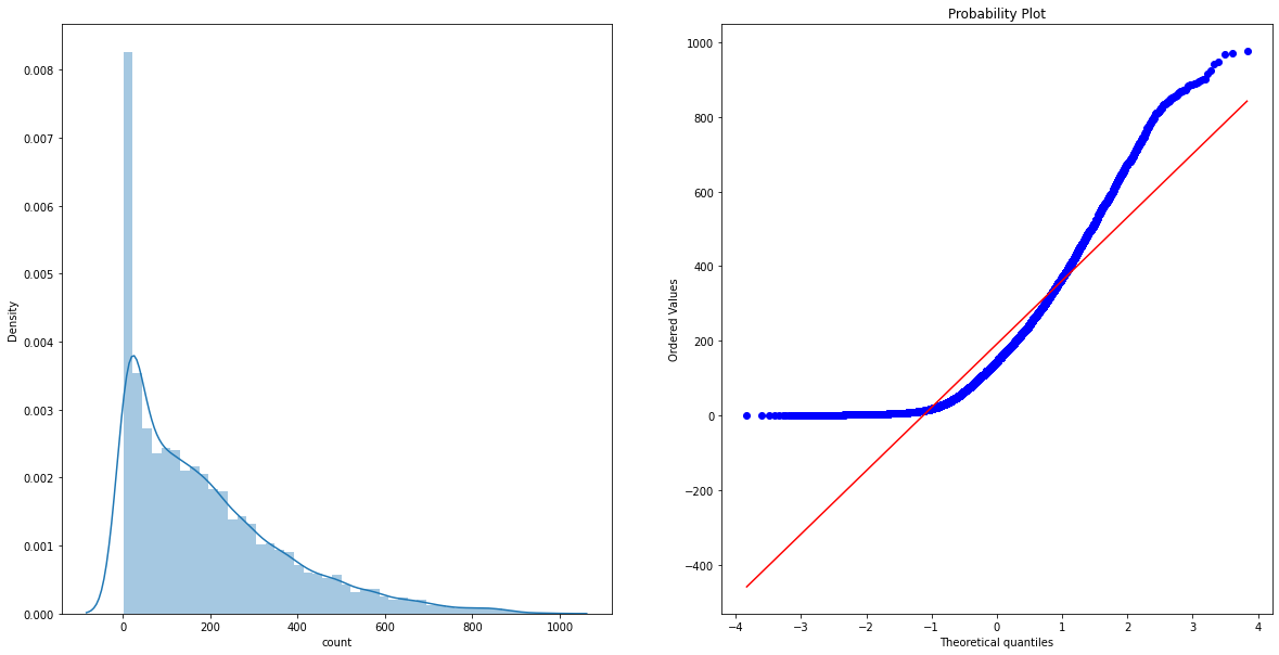
Skewness & Kurtosis
Skewness(왜도)와 Kurtosis(첨도)를 통해 데이터 분포의 치우침을 확인하고 보정한다.
print("Skewness: ", train['count'].skew())
print("Kurtosis: ", train['count'].kurt())
Skewness:  1.242066211718077
Kurtosis:  1.3000929518398299
fig, (ax1, ax2) = plt.subplots(ncols=2)
fig.set_size_inches(20, 10)

sns.distplot(train['count'], ax=ax1)
stats.probplot(train['count'], dist="norm", fit=True, plot=ax2)
/opt/conda/lib/python3.7/site-packages/seaborn/distributions.py:2619: FutureWarning: `distplot` is a deprecated function and will be removed in a future version. Please adapt your code to use either `displot` (a figure-level function with similar flexibility) or `histplot` (an axes-level function for histograms).
  warnings.warn(msg, FutureWarning)


((array([-3.83154229, -3.60754977, -3.48462983, ...,  3.48462983,
          3.60754977,  3.83154229]),
  array([  1,   1,   1, ..., 968, 970, 977])),
 (169.82942673231386, 191.5741319125482, 0.9372682766213176))
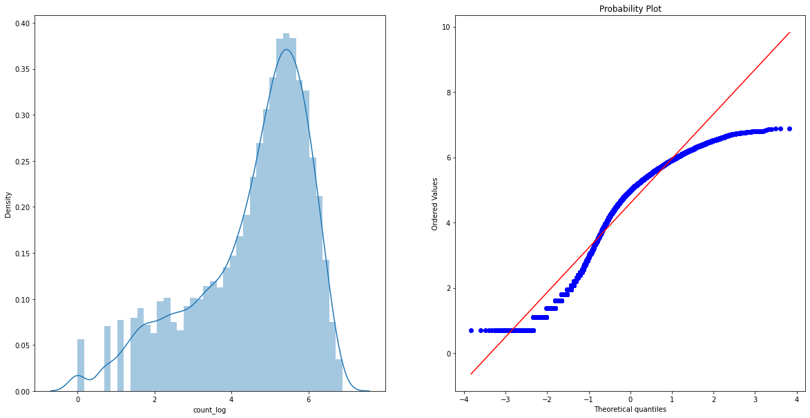
로그 스케일 정규화
Skewness의 쏠림이 있으므로 로그 스케일 정규화를 할 것이다.
train['count_log'] = np.log(train['count'])
print("Skewness: ", train['count_log'].skew())
print("Kurtosis: ", train['count_log'].kurt())
Skewness:  -0.9712277227866108
Kurtosis:  0.24662183416964067
fig, (ax1, ax2) = plt.subplots(ncols=2)
fig.set_size_inches(20, 10)

sns.distplot(train['count_log'], ax=ax1)
stats.probplot(np.log1p(train['count']), dist="norm", fit=True, plot=ax2)
/opt/conda/lib/python3.7/site-packages/seaborn/distributions.py:2619: FutureWarning: `distplot` is a deprecated function and will be removed in a future version. Please adapt your code to use either `displot` (a figure-level function with similar flexibility) or `histplot` (an axes-level function for histograms).
  warnings.warn(msg, FutureWarning)


((array([-3.83154229, -3.60754977, -3.48462983, ...,  3.48462983,
          3.60754977,  3.83154229]),
  array([0.69314718, 0.69314718, 0.69314718, ..., 6.87626461, 6.87832647,
         6.88550967])),
 (1.3647396459244172, 4.591363690454027, 0.9611793780126952))
One-hot encoding
print(train['weather'].unique())
print(train['season'].unique())
print(train['workingday'].unique())
print(train['holiday'].unique())
[2 1 3 4]
[1 2 3 4]
[0 1]
[0 1]
def one_hot_encoding(df):
    df = pd.get_dummies(df, columns=['weather'], prefix='weather')
    df = pd.get_dummies(df, columns=['season'], prefix='season')
    df = pd.get_dummies(df, columns=['workingday'], prefix='workingday')
    df = pd.get_dummies(df, columns=['holiday'], prefix='holiday')
    return df
train_before_encoding = train.copy()
train = one_hot_encoding(train)
train.columns
Index(['datetime', 'temp', 'atemp', 'humidity', 'windspeed', 'casual',
       'registered', 'count', 'season_str', 'year', 'month', 'day', 'weekday',
       'hour', 'count_log', 'weather_1', 'weather_2', 'weather_3', 'weather_4',
       'season_1', 'season_2', 'season_3', 'season_4', 'workingday_0',
       'workingday_1', 'holiday_0', 'holiday_1'],
      dtype='object')
상관관계 분석
## Pearson 상관계수 히트맵 시각화
fix, (ax1, ax2) = plt.subplots(figsize=(20, 30), nrows=2)
sns.heatmap(train_before_encoding.corr(), annot=True, fmt=".2f", cmap="BuPu", ax=ax1)
sns.heatmap(train.corr(), annot=True, fmt=".2f", cmap="Blues", ax=ax2)
<AxesSubplot:>
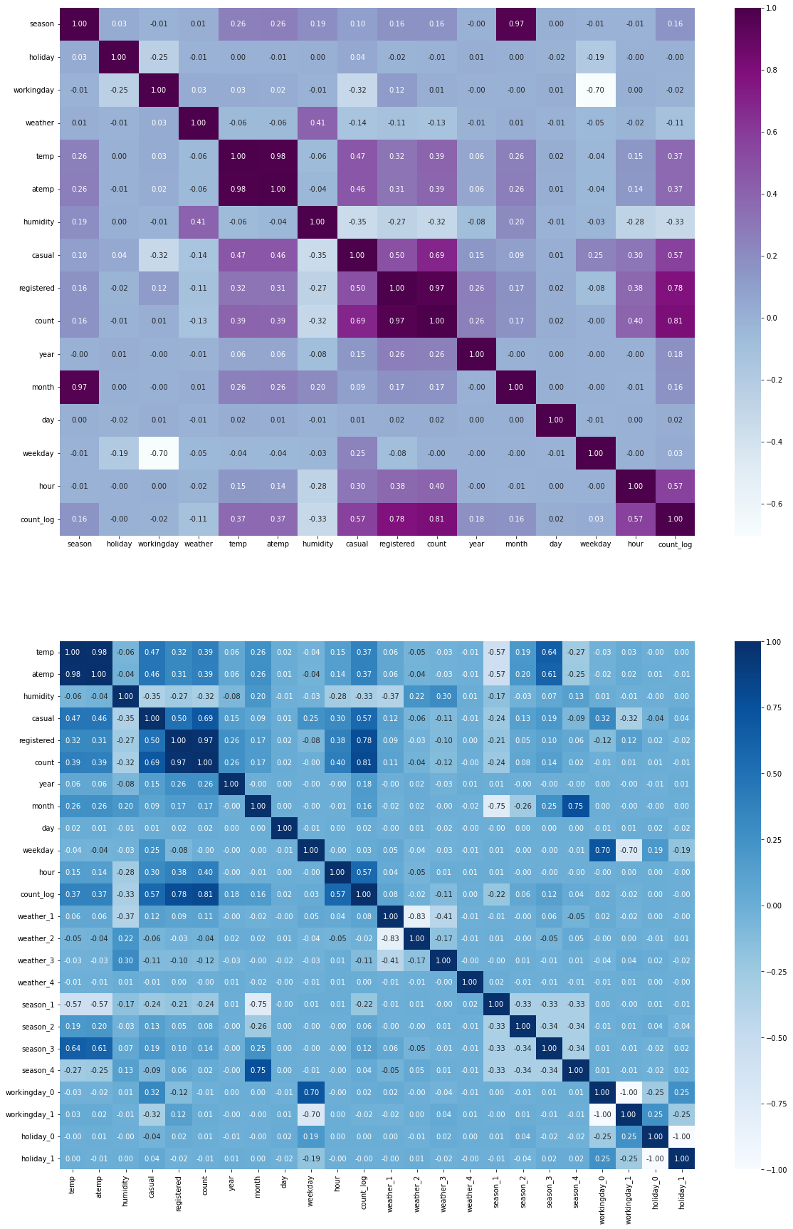
## count와의 상관계수 절대값 내림차순
corr = train.corr()[['count']]
corr.rename(columns={'count': 'corr'}, inplace=True)
corr['corr_abs'] = corr['corr'].abs()
corr.sort_values(by='corr_abs', ascending=False)
| corr | corr_abs | |
|---|---|---|
| count | 1.000000 | 1.000000 |
| registered | 0.970948 | 0.970948 |
| count_log | 0.805773 | 0.805773 |
| casual | 0.690414 | 0.690414 |
| hour | 0.400601 | 0.400601 |
| temp | 0.394454 | 0.394454 |
| atemp | 0.389784 | 0.389784 |
| humidity | -0.317371 | 0.317371 |
| year | 0.260403 | 0.260403 |
| season_1 | -0.237704 | 0.237704 |
| month | 0.166862 | 0.166862 |
| season_3 | 0.136942 | 0.136942 |
| weather_3 | -0.117519 | 0.117519 |
| weather_1 | 0.105246 | 0.105246 |
| season_2 | 0.075681 | 0.075681 |
| weather_2 | -0.041329 | 0.041329 |
| season_4 | 0.023704 | 0.023704 |
| day | 0.019826 | 0.019826 |
| workingday_1 | 0.011594 | 0.011594 |
| workingday_0 | -0.011594 | 0.011594 |
| holiday_1 | -0.005393 | 0.005393 |
| holiday_0 | 0.005393 | 0.005393 |
| weekday | -0.002283 | 0.002283 |
| weather_4 | -0.001459 | 0.001459 |
모델
피처 엔지니어링
EDA 과정에서 Train 데이터에 행한 과정을 Test 데이터에도 적용한다.
test = build_datetime_features(test)
test = predict_windspeed(test)
test = one_hot_encoding(test)
/opt/conda/lib/python3.7/site-packages/ipykernel_launcher.py:10: SettingWithCopyWarning:
A value is trying to be set on a copy of a slice from a DataFrame.
Try using .loc[row_indexer,col_indexer] = value instead

See the caveats in the documentation: https://pandas.pydata.org/pandas-docs/stable/user_guide/indexing.html#returning-a-view-versus-a-copy
  ## Remove the CWD from sys.path while we load stuff.
test.head()
| datetime | temp | atemp | humidity | windspeed | season_str | year | month | day | weekday | ... | weather_3 | weather_4 | season_1 | season_2 | season_3 | season_4 | workingday_0 | workingday_1 | holiday_0 | holiday_1 | |
|---|---|---|---|---|---|---|---|---|---|---|---|---|---|---|---|---|---|---|---|---|---|
| 0 | 2011-01-20 00:00:00 | 10.66 | 11.365 | 56 | 26.0027 | Spring | 2011 | 1 | 20 | 3 | ... | 0 | 0 | 1 | 0 | 0 | 0 | 0 | 1 | 1 | 0 |
| 1 | 2011-01-20 03:00:00 | 10.66 | 12.880 | 56 | 11.0014 | Spring | 2011 | 1 | 20 | 3 | ... | 0 | 0 | 1 | 0 | 0 | 0 | 0 | 1 | 1 | 0 |
| 2 | 2011-01-20 04:00:00 | 10.66 | 12.880 | 56 | 11.0014 | Spring | 2011 | 1 | 20 | 3 | ... | 0 | 0 | 1 | 0 | 0 | 0 | 0 | 1 | 1 | 0 |
| 3 | 2011-01-20 05:00:00 | 9.84 | 11.365 | 60 | 15.0013 | Spring | 2011 | 1 | 20 | 3 | ... | 0 | 0 | 1 | 0 | 0 | 0 | 0 | 1 | 1 | 0 |
| 4 | 2011-01-20 06:00:00 | 9.02 | 10.605 | 60 | 15.0013 | Spring | 2011 | 1 | 20 | 3 | ... | 0 | 0 | 1 | 0 | 0 | 0 | 0 | 1 | 1 | 0 |
5 rows × 23 columns
필드 선택
count와 상관계수가 높은 필드- 의미가 중복되는 컬럼은 덜 분산된 필드 선택
- ex.
workingday와holiday는 부의 상관관계가 있으나,workingday의 분산이 작으므로workingday선택
- ex.
test_datetime = test['datetime']
train.drop(['datetime', 'season_str', 'holiday_0', 'holiday_1', 'atemp', 'registered', 'casual'], axis=1, inplace=True)
test.drop(['datetime', 'season_str', 'holiday_0', 'holiday_1', 'atemp'], axis=1, inplace=True)
print(train.columns)
print(test.columns)
Index(['temp', 'humidity', 'windspeed', 'count', 'year', 'month', 'day',
       'weekday', 'hour', 'count_log', 'weather_1', 'weather_2', 'weather_3',
       'weather_4', 'season_1', 'season_2', 'season_3', 'season_4',
       'workingday_0', 'workingday_1'],
      dtype='object')
Index(['temp', 'humidity', 'windspeed', 'year', 'month', 'day', 'weekday',
       'hour', 'weather_1', 'weather_2', 'weather_3', 'weather_4', 'season_1',
       'season_2', 'season_3', 'season_4', 'workingday_0', 'workingday_1'],
      dtype='object')
Gradient boosting
from sklearn.model_selection import train_test_split
from sklearn.ensemble import GradientBoostingRegressor
from sklearn import metrics
x_train = train.drop(['count_log', 'count'], axis=1).values
target_label = train['count_log'].values
x_test = test.values
x_train, x_val, y_train, y_val = train_test_split(x_train, target_label, test_size=0.2, random_state=2000)
x_train
array([[14.76, 50, 16.9979, ..., 1, 0, 1],
       [33.62, 43, 19.9995, ..., 0, 1, 0],
       [31.16, 58, 19.0012, ..., 0, 0, 1],
       ...,
       [22.96, 37, 19.0012, ..., 0, 0, 1],
       [18.86, 63, 8.9981, ..., 1, 0, 1],
       [17.22, 38, 19.9995, ..., 0, 0, 1]], dtype=object)
gbr_model = GradientBoostingRegressor(
    n_estimators=2000,
    learning_rate=0.05,
    max_depth=5,
    min_samples_leaf=15,
    min_samples_split=10,
    random_state=42
)
gbr_model.fit(x_train, y_train)
GradientBoostingRegressor(learning_rate=0.05, max_depth=5, min_samples_leaf=15,
                          min_samples_split=10, n_estimators=2000,
                          random_state=42)
Validation
train_score = gbr_model.score(x_train, y_train)
validation_score = gbr_model.score(x_val, y_val)
print(train_score, validation_score)
0.9866447588995861 0.957037659130984
자전거 수요 예측
gbr_prediction = gbr_model.predict(x_test)
predicted_count = np.exp(gbr_prediction)
sample.head()
| datetime | count | |
|---|---|---|
| 0 | 2011-01-20 00:00:00 | 0 |
| 1 | 2011-01-20 01:00:00 | 0 |
| 2 | 2011-01-20 02:00:00 | 0 |
| 3 | 2011-01-20 03:00:00 | 0 |
| 4 | 2011-01-20 04:00:00 | 0 |
submission = pd.DataFrame()
submission['datetime'] = test_datetime
submission['count'] = predicted_count
submission.head()
| datetime | count | |
|---|---|---|
| 0 | 2011-01-20 00:00:00 | 13.892524 |
| 1 | 2011-01-20 03:00:00 | 2.242351 |
| 2 | 2011-01-20 04:00:00 | 2.509201 |
| 3 | 2011-01-20 05:00:00 | 5.775774 |
| 4 | 2011-01-20 06:00:00 | 31.641682 |
submission.to_csv("bike.csv", index=False)